Lah-Laguerre Optics
Published in arXiv:2011, 30 October 2020
Published in Optics Express 30, 22, 20 October 2022
Operating with ultrashort, broadband laser pulses presents a challenge to maintain the pulse phase intact so that the pulse duration or shape does not change and the peak power does not decrease substantially.
 |
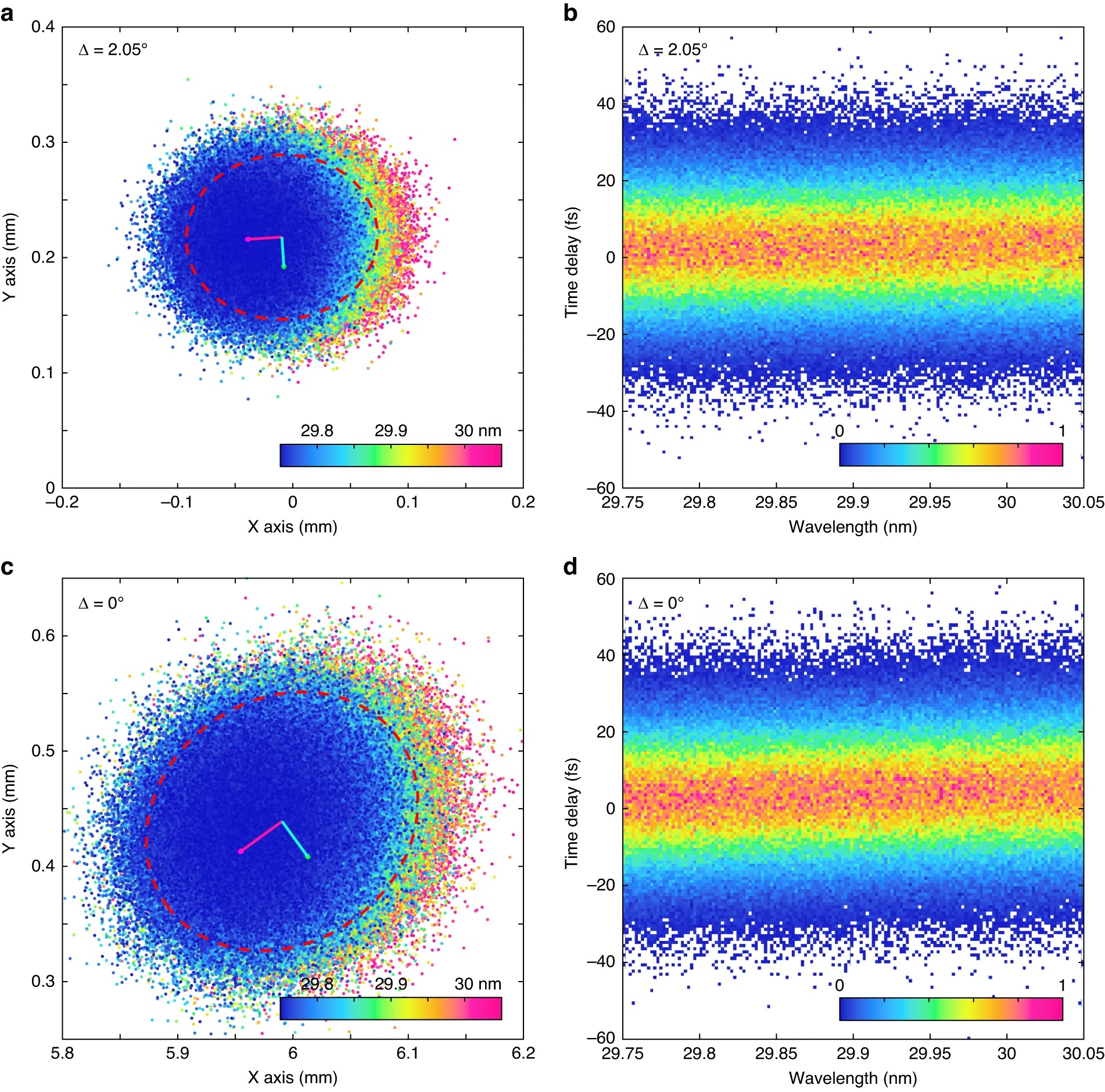
| Ultrashort pulse stemming from an anti-resonant fiber |
The description of uniform systems allows for the exact implementation of the accumulated phase, i.e., pulse propagation in waveguides or optical fibers. However, balancing the pulse phase becomes an optimization problem when several systems are interconnected. It is no longer practical due to computational speed to match phases ‘shapes’ but rather individual perturbative orders of dispersion. The cited papers have lay the foundation of analytical and more robust description for the chromatic dispersion phenomena that will aid the design of novel optical systems and materials.
The perturbative description of the chromatic dispersion involves several hypergeometrical transforms, the most famous amongst, are the Lah, and Laguerre transforms. The Lah, Laguerre, and several other unnamed forward and inverse transforms form the core of the Lah-Laguerre dispersive optics. In Lah-Laguerre optics, such algorithms allow for incredibly faster computations when solving complicated optimization problems involving phase balancing of different optical systems, at the extereme single cycle waform synthesis.
Using the Lah-Laguerre approach gives the mathematical foundation to evaluate, optimize, and design systems, to output a pulse desired pulse duration balanced to an anticipated chromatic dispersion order. However, due to the experimental uncertainty in measurements of the refractive index or due to the simplified level of description of an optical system, these relations can leave some ambiguity in the estimated chromatic dispersion orders. Fortunately, the inverse transforms relate the Taylor coefficients of the refractive index or optical path to the phase or wavevector. Thus, to put in perspective, a single point phase measurement, provides information for the refractive index or optical path in an extended vicinity of measured frequency. Consequently, this formalism can also facilitate more precise interferometric measurements of the refractive index and aid the design of novel optical materials, nanostructures, and optical systems based on desired dispersion. Furthermore, from a practical point of view, the evaluation speed of the simple hypergeometric series can be competitive even against algorithms such as the fast Fourier transform (FFT). Numerically, the highest order that can be evaluated is solely limited by the computer architecture’s ability to allocate the smallest /largest/ floating-point number.
When pulses have substantial bandwidth it is essential to consider also the higher orders of dispersion. A few example of evaluated chromatic dispersion orders follow below.
The first 10 material dispersion orders of \(CaF_2\) material are shown below. More data plots for the material dispersion orders of various materials can be found in Ref.[2].
 |
Material dispersion orders for \(CaF_2\)
|
The first 10 chromatic dispersion orders of conventional genuine laser pulse compressors are illustrated below.
 |
| Chromatic dispersion orders in A) grating compressor B) Prism-pair compressor | | |
For more information, please visit the original papers Ref [1], Ref [2], Ref [3].
Mathematical description.
In dispersive systems, the phase velocity of a wave depends on its
frequency. Effectively a single wavelength monochromatic light will accumulate
phase and will experience a time delay compared to the same wave traveling in a
vacuum. Such idealized waves have infinite pulse duration – continuous waves. In
contrast, when considering many monochromatic waves that interfere constructively
over a small spatial extent, create a wavepacket that will experience more
dramatic changes. In such cases, we can define a group delay and group
velocity dispersion that is a result of collective behavior of the wavelets. The propagation of pulses in matter leads to changes
in the phase and pulse duration. In linear light-matter interactions, the
spectrum of the wavepacket does not change. The phenomenon is known as
chromatic dispersion. The chromatic dispersion has worked both in favor and
against some of the most significant innovations of the
past decades.
The dispersion relation for the phase is:
\(\begin{array}{c}\varphi\hspace{-0.5mm}\left(\omega|\lambda \right) = k \hspace{-0.1mm}\mathrm{(}\omega\mathrm{)}z = \frac{\omega}{c}n \mathrm{(}\omega\mathrm{)}z = \frac{2\pi}{\lambda}n \mathrm{(}\lambda\mathrm{)}z = \frac{\omega}{c}{\it OP} \mathrm{(}\omega\mathrm{)} = \frac{2\pi}{\lambda}{\it OP} \mathrm{(}\lambda\mathrm{)} = \omega\tau \mathrm{(}\omega\mathrm{)} = \frac{2\pi}{\tau_{0}}\tau \mathrm{(}\omega\mathrm{)} \tag{1}\label{myeq1} \end{array} \)
where \({\it OP}\mathrm{(}\omega \mathrm{|}\lambda \mathrm{)}\) is the optical path, \(n\mathrm{(}\omega \mathrm{|}\lambda \mathrm{)}\) is the refractive index of the medium, \(\tau \mathrm{(}\omega \mathrm{|}\lambda \mathrm{)}\) is the corresponding temporal interval, and \({\tau }_0\mathrm{\ }\) is the single-cycle pulse duration for a wavelet with a wavelength \(\lambda \). In such a picture, the spectral content of the signal does not change but rather rearranges temporally over a certain band around an average frequency \({\omega }_0\). Historically, the dispersion orders have been defined in the frequency space through the Taylor expansion of the phase \(\varphi \mathrm{(}\omega \mathrm{|}\lambda \mathrm{)}\), or the wavevector \(k\hspace{-0.1mm} \mathrm{(}\omega \mathrm{|}\lambda \mathrm{)}\) around the pulse intensity-averaged frequency or the carrier frequency at the pulse peak
The dispersion orders are defined by the Taylor expansion of the phase or the wavevector.
\( \begin{array}{c}\varphi \mathrm{(}\omega\mathrm{)} = \varphi\hspace{-1.5mm}\left.\ \right|_{\omega_{0}} + \left. \ \frac{\partial\varphi}{\partial\omega} \right|_{\omega_{0}} \hspace{-1.0mm}\left(\omega - \omega_{0} \right) + \frac{1}{2}\hspace{-1.3mm}\left. \ \frac{\partial^{\hspace{0.3pt}{2}}\varphi}{\partial\omega^{2}} \right|_{\omega_{0}} \hspace{-1.0mm}\left(\omega - \omega_{0} \right)^{2}\ + \ldots + \frac{1}{p!}\hspace{0.0mm}\left. \ \frac{\partial^{\hspace{0.1pt}{p}}\varphi}{\partial\omega^{p}} \right|_{\omega_{0}} \hspace{-1.0mm}\left(\omega - \omega_{0} \right)^{p} + \ldots = \end{array}\)
\(\begin{array}{c}= \varphi \hspace{-1.6mm} \left. \ \right|_{\omega_{0}} + \tau_{g} \hspace{-1.9mm} \left. \ \right|_{\omega_{0}}\hspace{0.0mm}\left( \omega - \omega_{0} \right) + \frac{1}{2}{\it GDD}\hspace{0.0mm}\left( \omega - \omega_{0} \right)^{2} + \ldots + \frac{1}{p!}{\it POD}\hspace{0.0mm}\left( \omega - \omega_{0} \right)^{p} + \mathrm{\it{R_p}} \tag{2}\label{myeq2} \end{array}\)
Such a representation is convenient as it requires knowledge only of a small number of spectral derivatives at a single point. The first derivative \({\left.\frac{\partial \varphi }{\partial \omega }\right|}_{{\omega }_0} \hspace{-0.9mm}= {\tau }_g\) corresponds to the group delay (\({\it GD}\)), which results in a temporal lag of the pulse envelope. The presence of higher orders causes distortions in the temporal pulse shape. The second term \({\left.\frac{{\partial }^{\hspace{0.3pt}{2}}\varphi }{\partial {\omega }^{\mathrm{2}}}\right|}_{{\omega }_0} \hspace{-0.9mm}= {\left.\frac{\partial }{\partial \omega }{\tau }_g \hspace{-0.2mm} \mathrm{(}\omega \mathrm{)}\right|}_{{\omega }_0}\)corresponds to the group delay dispersion (\({\it GDD}\)), and in general, \({\left.\frac{{\partial }^{\hspace{0.1pt}{p}}\varphi }{\partial {\omega }^p}\right|}_{{\omega }_0} = {\left.\frac{{\partial }^{p\mathrm{-}\mathrm{1}}}{\partial {\omega }^{p\mathrm{-}\mathrm{1}}}{\tau }_g \hspace{-0.2mm} \mathrm{(}\omega \mathrm{)}\right|}_{{\omega }_0}\) is the \(p^{t\hspace{-0.3mm}h}\) order dispersion (\({\it POD}\)). Finally, \(R_{p} = \mathop{max}\limits_{\omega \leq \xi \leq \omega_{0}}\frac{\partial^{p + 1}\varphi(\xi)}{\partial\xi^{p + 1}}\frac{{\ \left( \omega - \omega_{0} \right)}^{p + 1}}{(p + 1)!}
\) is the Lagrange error after the first \({\it{p}}\) terms.
In a similar fashion, the wavevector \(k \hspace{-0.1mm}\mathrm{(}\omega \mathrm{|}\lambda \mathrm{)}\) can be expanded in a Taylor series :
\(\begin{array}{c}k\hspace{-0.1mm} \mathrm{(}\omega \mathrm{)}=k{\left.{}\right|}_{{\omega }_0}+{\left.\frac{\partial k}{\partial \omega }\right|}_{{\omega }_0}\hspace{-0.85mm}\left(\omega -{\omega }_0\right)+\frac{1}{2}{\left.\frac{{\partial }^2k}{\partial {\omega }^2}\right|}_{{\omega }_0}\hspace{-0.75mm}{\left(\omega -{\omega }_0\right)}^2\ +\dots +\frac{1}{p!}{\left.\frac{{\partial }^{\hspace{0.1pt}{p}}k}{\partial {\omega }^p}\right|}_{{\omega }_0}\hspace{-0.3mm}{\left(\omega -{\omega }_0\right)}^p+\dots=\end{array}
\)
\( \begin{array}{c}
=k_0+v^{-1}_{gr}\hspace{-0.5mm}\left(\omega -{\omega }_0\right)+\frac{1}{2}{\it GDD}{\left(\omega -{\omega }_0\right)}^2+\dots +\frac{1}{p!}{\it POD}{\left(\omega -{\omega }_0\right)}^p+\mathrm{\it{R_p}} \tag{3}\label{myeq3} \end{array}
\)
Again, the lowest term \({\left.\frac{\partial k}{\partial \omega
}\right|}_{{\omega }_0} \hspace{-0.9mm}=\hspace{-0.3mm}
\frac{\mathrm{1}}{v_g} \hspace{-0.3mm}=\hspace{-0.3mm} \frac{{\tau
}_g}{z}\) represents the inverse group velocity, whereas the second term
\({\left.\frac{{\partial }^{\hspace{0.3pt}{2}}k}{\partial {\omega
}^{\mathrm{2}}}\right|}_{{\omega }_0} \hspace{-1.0mm}=
{\left.\frac{\partial }{\partial \omega
}v^{\mathrm{-}\mathrm{1}}_{gr}\right|}_{{\omega }_0}\) represents the
\({\it GDD}\). In general, \({\left.\frac{{\partial
}^{\hspace{0.1pt}{p}}k}{\partial {\omega }^p}\right|}_{{\omega }_0}
\hspace{-0.9mm}= {\left.\frac{{\partial
}^{p\mathrm{-}\mathrm{1}}}{\partial {\omega
}^{p\mathrm{-}\mathrm{1}}}v^{\mathrm{-}\mathrm{1}}_{gr}\right|}_{{\omega
}_0}\) is the \(p^{t\hspace{-0.3mm}h}\) order dispersion (\({\it
POD}\)).
The chromatic dispersion orders can be easily evaluated in the frequency domain by obtaining the successive derivatives of the wavevector \(k\hspace{-0.1mm}\mathrm{(}\omega \mathrm{)}\) or the phase \(\varphi \mathrm{(}\omega \mathrm{)}\). In general:
\( \begin{array}{c}\frac{{\partial }^{\hspace{0.1pt}{p}}}{\partial {\omega }^p}k \mathrm{(}\omega \mathrm{)}=\frac{1}{c}\left(p\frac{{\partial }^{p-1}}{\partial {\omega }^{p-1}}n \mathrm{(}\omega \mathrm{)}+\omega \frac{{\partial }^{\hspace{0.1pt}{p}}}{\partial {\omega }^p}n \mathrm{(}\omega \mathrm{)}\right) \tag{4}\label{myeq4} \end{array}\)
\(\begin{array}{c}
\frac{{\partial }^{\hspace{0.1pt}{p}}}{\partial {\omega }^p}\varphi \mathrm{(}\omega \mathrm{)} = \frac{1}{c}\left(p\frac{{\partial }^{p-1}}{\partial {\omega }^{p-1}}{\it OP} \mathrm{(}\omega \mathrm{)}+\omega \frac{{\partial }^{\hspace{0.1pt}{p}}}{\partial {\omega }^p}{\it OP} \mathrm{(}\omega \mathrm{)}\right) \tag{5}\label{myeq5} \end{array}
\)
The derivatives of any differentiable function \(f\mathrm{(}\omega \mathrm{|}\lambda \mathrm{)}\) in the
wavelength or the frequency space is specified through a Lah transform as:
\( \begin{array}{c} \text{}\hspace{2pt}
\frac{{\partial }^{\hspace{0.1pt}{p}}}{\partial {\omega }^p}f \mathrm{(}\omega \mathrm{)}={}{\left(\mathrm{-}\mathrm{1}\right)}^p{\left(\frac{\lambda }{\mathrm{2}\pi c}\right)}^p\sum\limits^p_{m = {0}}{\mathcal{A}\hspace{0.0mm}\mathrm{(}p,m\mathrm{)}\hspace{0.3mm}{\lambda }^m\frac{{\partial }^{\hspace{0.3pt}{m}}}{\partial {\lambda }^m}f \mathrm{(}\lambda \mathrm{)}}
\tag{6}\label{myeq6} \end{array} \hspace{-1.5em}\)
\( \begin{array}{c} \text{}\hspace{2pt}
\frac{{\partial }^{\hspace{0.1pt}{p}}}{\partial {\lambda }^p}f \mathrm{(}\lambda \mathrm{)}={}{\left(\mathrm{-}\mathrm{1}\right)}^p{\left(\frac{\omega }{\mathrm{2}\pi c}\right)}^p\sum\limits^p_{m = {0}}{\mathcal{A}\hspace{0.0mm}\mathrm{(}p,m\mathrm{)}\hspace{0.3mm}{\omega }^m\frac{{\partial }^{\hspace{0.3pt}{m}}}{\partial {\omega }^m}f \mathrm{(}\omega \mathrm{)}}\tag{7}\label{myeq7} \end{array} \hspace{-1.5em}\)
The matrix elements of the transformation are
the Lah coefficients: \(\mathcal{A}\mathrm{(}p,m\mathrm{)} = \frac{p\mathrm{!}}{\left(p\mathrm{-}m\right)\mathrm{!}m\mathrm{!}}\frac{\mathrm{(}p\mathrm{-}\mathrm{1)!}}{\mathrm{(}m\mathrm{-}\mathrm{1)!}}\)
Written for the \({\it GDD}\) the above expression states
that a constant with wavelength \({\it GDD}\), will have zero higher orders. From a practical point of view, when the \({\it GDD}\) data is experimentally or numerically accessible in the wavelength space, the dispersion orders can be expressed as:
\( \begin{array}{c}
\frac{{\partial }^{p+2}}{\partial {\omega }^{p+2}} \varphi \mathrm{(}\omega \mathrm{)}=\frac{{\partial }^{\hspace{0.1pt}{p}}}{\partial {\omega }^p} {\it GDD}={\left(-1\right)}^p{\left(\frac{\lambda }{2\pi c}\right)}^p\sum\limits^p_{m=0}{\mathcal{A}\hspace{0.0mm}\mathrm{(}p,m\mathrm{)}\ {\lambda }^m\frac{{\partial }^{\hspace{0.3pt}{m}}}{\partial {\lambda }^m}{\it GDD} \mathrm{(}\lambda \mathrm{)}}\tag{8}\label{myeq8} \end{array}
\)
Substituting equation (6) and (7) expressed for the
refractive index \(n\) or optical path \(OP\) into equation (4) and (5) results in closed-form
expressions for the dispersion orders. In general the \(p^{th}\) order
dispersion (\({\it POD}\)) is a Laguerre type transform of negative order two:
\( \begin{array}{c}\text{}\hspace{2pt}{\it POD}\mathrm{(}n \mathrm{)}=\frac{{\partial }^{\hspace{0.1pt}{p}}}{\partial {\omega }^p} k \mathrm{(}\omega \mathrm{)}={\left(-1\right)}^p\frac{1}{c}{\left(\frac{\lambda }{2\pi c}\right)}^{p-1}\sum\limits^p_{m=0}{\mathcal{B}\hspace{0.0mm}\mathrm{(}p,m\mathrm{)}\ {\lambda }^m\frac{{\partial }^{\hspace{0.3pt}{m}}}{\partial {\lambda }^m}n \mathrm{(}\lambda \mathrm{)}} \tag{9}\label{myeq9} \end{array} \)
\( \begin{array}{c}\text{}\hspace{2pt}{\it POD}\mathrm{(}{\it OP} \mathrm{)}=\frac{{\partial }^{\hspace{0.1pt}{p}}}{\partial {\omega }^p} \varphi \mathrm{(}\omega \mathrm{)}={\left(-1\right)}^p\frac{1}{c}{\left(\frac{\lambda }{2\pi c}\right)}^{p-1}\sum\limits^p_{m=0}{\mathcal{B}\hspace{0.0mm}\mathrm{(}p,m\mathrm{)}\ {\lambda }^m\frac{{\partial }^{\hspace{0.3pt}{m}}}{\partial {\lambda }^m}{\it OP} \mathrm{(}\lambda \mathrm{)}} \tag{10}\label{myeq10} \end{array} \)
The inverse transforms relate the Taylor coefficients of the refractive index or the optical path to the wavevector or the phase.
\(\begin{array}{c}\text{}\hspace{2pt}{\lambda }^p\frac{{\partial }^{\hspace{0.1pt}{p}}}{\partial {\lambda }^p}n \mathrm{(}\lambda \mathrm{)}={\left(-1\right)}^p\frac{c}{\omega }\sum\limits^p_{m=0}{\mathcal{B}\hspace{0.0mm}\mathrm{(}p,m\mathrm{)}\hspace{0.5mm}{\omega }^m\frac{{\partial }^{\hspace{0.3pt}{m}}}{\partial {\omega }^m} k \mathrm{(}\omega \mathrm{)} }\tag{11}\label{myeq11} \end{array}\)
\(\begin{array}{c}\text{}\hspace{2pt}{\lambda }^p\frac{{\partial }^{\hspace{0.1pt}{p}}}{\partial {\lambda }^p}{\it OP} \mathrm{(}\lambda \mathrm{)}={\left(-1\right)}^p\frac{c}{\omega }\sum\limits^p_{m=0}{\mathcal{B}\hspace{0.0mm}\mathrm{(}p,m\mathrm{)}\hspace{0.5mm}{\omega }^m\frac{{\partial }^{\hspace{0.3pt}{m}}}{\partial {\omega }^m} \varphi \mathrm{(}\omega \mathrm{)}\ }\tag{12}\label{myeq12} \end{array}\)
The matrix elements of the transforms are the unsigned Laguerre coefficients of order negative two: \(\mathcal{B}\hspace{0.0mm}\mathrm{(}p,m\mathrm{)} = \frac{p\mathrm{!}}{\left(p\mathrm{-}m\right)\mathrm{!}m\mathrm{!}}\frac{\mathrm{(}p\mathrm{-}\mathrm{2)!}}{\mathrm{(}m\mathrm{-}\mathrm{2)!}}\)
The polynomial sums form sequential polynomials \(G^{\left(\alpha \right)}_p\mathrm{(}x\mathrm{)}\) . The corresponding generating function can be expressed as:
\( \begin{array}{c}
G^{ \left(\alpha \right)}_p\mathrm{(}x\mathrm{)}=x^{-\alpha }\frac{d^p}{dx^p}\left(x^{p+\alpha }f \mathrm{(}x\mathrm{)}\right)=\sum\limits^p_{m=0}{\mathcal{C}\mathrm{(}p+\alpha ,p-m\mathrm{)}\frac{p!}{m!}x^m}f^{\left(m\right)} \mathrm{(}x\mathrm{)}\tag{13}\label{myeq13} \end{array}
\)
The first four chromatic dispersion orders are well-known in the literature. Using the above-mentioned Lah-Laguerre optical formalism, the first ten dispersion orders, written for the wavevector, can be explicitly written in closed-form expressions as:
\(\begin{array}{l}\hspace{-55pt}\text{C I}.\hspace{2pt}\boldsymbol{{\it GD}} = \frac{\partial }{\partial \omega }k\hspace{-0.3mm} \mathrm{(}\omega \mathrm{)} = \frac{\mathrm{1}}{c}\left(n \mathrm{(}\omega \mathrm{)}+\omega \frac{\partial n \mathrm{(}\omega \mathrm{)}}{\partial \omega }\right) = {-}\frac{\mathrm{1}}{c}G^{\left(\mathrm{-}\mathrm{2}\right)}_{\mathrm{1}} \mathrm{(}\lambda \mathrm{)}=\frac{\mathrm{1}}{c}\left(n \mathrm{(}\lambda \mathrm{)}-\lambda \frac{\partial n \mathrm{(}\lambda \mathrm{)}}{\partial\lambda }\right) = v^{\mathrm{-}\mathrm{1}}_{gr}\tag{14}\label{myeq14} \end{array} \hspace{-0.5em}\)
The group refractive index \(n_g\)is defined in terms of the group velocity \(v_{gr}\): \(n_g\enspace = \enspace cv^{\mathrm{-}\mathrm{1}}_{gr}\).
\(\begin{array}{l}\hspace{-115pt}\text{C II}.\hspace{2pt}\boldsymbol{{\it GDD}} = \frac{{\partial }^{\hspace{0.3pt}{2}}}{\partial {\omega }^{\mathrm{2}}}k\hspace{-0.3mm} \mathrm{(}\omega \mathrm{)} = \frac{\mathrm{1}}{c}\left(\mathrm{2}\frac{\partial n\mathrm{(}\omega \mathrm{)}}{\partial \omega }+\omega \frac{{\partial }^{\hspace{0.3pt}{2}}n\mathrm{(}\omega \mathrm{)}}{\partial {\omega }^{\mathrm{2}}}\right) = \frac{\mathrm{1}}{c}\left(\frac{\lambda }{\mathrm{2}\pi c}\right)G^{\left(\mathrm{-}\mathrm{2}\right)}_{\mathrm{2}} \mathrm{(}\lambda \mathrm{)} = \\= \frac{\mathrm{1}}{c}\left(\frac{\lambda }{\mathrm{2}\pi c}\right)\left({\lambda }^{\mathrm{2}}\frac{{\partial }^{\hspace{0.3pt}{2}}n \mathrm{(}\lambda \mathrm{)}}{\partial {\lambda }^{\mathrm{2}}}\right)\tag{15}\label{myeq15} \end{array} \hspace{-0.5em}\)
\(\begin{array}{l}\hspace{-99pt}\text{C III}.\hspace{2pt}\boldsymbol{{\it TOD}} = \frac{{\partial }^{\hspace{0.3pt}{3}}}{\partial {\omega }^{\mathrm{3}}}k\hspace{-0.3mm} \mathrm{(}\omega \mathrm{)} = \frac{\mathrm{1}}{c}\left(\mathrm{3}\frac{{\partial }^{\hspace{0.3pt}{2}}n\mathrm{(}\omega \mathrm{)}}{\partial {\omega }^{\mathrm{2}}}+\omega \frac{{\partial }^{\hspace{0.3pt}{3}}n\mathrm{(}\omega \mathrm{)}}{\partial {\omega }^{\mathrm{3}}}\right) = {-}\frac{\mathrm{1}}{c}{\left(\frac{\lambda }{\mathrm{2}\pi c}\right)}^{\mathrm{2}}G^{\left(\mathrm{-}\mathrm{2}\right)}_{\mathrm{3}} \mathrm{(}\lambda \mathrm{)} = \\ = {-} \frac{\mathrm{1}}{c}{\left(\frac{\lambda }{\mathrm{2}\pi c}\right)}^{\mathrm{2}}\Bigl(\mathrm{3}{\lambda }^{\mathrm{2}}\frac{{\partial }^{\hspace{0.3pt}{2}}n \mathrm{(}\lambda \mathrm{)}}{\partial {\lambda }^{\mathrm{2}}} +{\lambda }^{\mathrm{3}}\frac{{\partial }^{\hspace{0.3pt}{3}}n \mathrm{(}\lambda \mathrm{)}}{\partial {\lambda }^{\mathrm{3}}}\Bigr)\tag{16}\label{myeq16} \end{array} \hspace{-0.5em}\)
\(\begin{array}{l}\hspace{-102pt}\text{C IV}.\hspace{2pt}\boldsymbol{{\it FOD}} = \frac{{\partial }^{\hspace{0.3pt}{4}}}{\partial {\omega }^{\mathrm{4}}}k\hspace{-0.3mm} \mathrm{(}\omega \mathrm{)} = \frac{\mathrm{1}}{c}\left(\mathrm{4}\frac{{\partial }^{\hspace{0.3pt}{3}}n\mathrm{(}\omega \mathrm{)}}{\partial {\omega }^{\mathrm{3}}}+\omega \frac{{\partial }^{\hspace{0.3pt}{4}}n\mathrm{(}\omega \mathrm{)}}{\partial {\omega }^{\mathrm{4}}}\right) = \frac{\mathrm{1}}{c}{\left(\frac{\lambda }{\mathrm{2}\pi c}\right)}^{\mathrm{3}}G^{\left(\mathrm{-}\mathrm{2}\right)}_{\mathrm{4}} \mathrm{(}\lambda \mathrm{)} = \\ = \frac{\mathrm{1}}{c}{\left(\frac{\lambda }{\mathrm{2}\pi c}\right)}^{\mathrm{3}}\Bigl(\mathrm{12}{\lambda }^{\mathrm{2}}\frac{{\partial }^{\hspace{0.3pt}{2}}n \mathrm{(}\lambda \mathrm{)}}{\partial {\lambda }^{\mathrm{2}}} +\mathrm{8}{\lambda }^{\mathrm{3}}\frac{{\partial }^{\hspace{0.3pt}{3}}n \mathrm{(}\lambda \mathrm{)}}{\partial {\lambda }^{\mathrm{3}}}+{\lambda }^{\mathrm{4}}\frac{{\partial }^{\hspace{0.3pt}{4}}n \mathrm{(}\lambda \mathrm{)}}{\partial {\lambda }^{\mathrm{4}}}\Bigr)\tag{17}\label{myeq17} \end{array} \hspace{-0.5em}\)
\(\begin{array}{l}\hspace{-67pt}\text{C V}.\hspace{2pt}\boldsymbol{{\it FiOD}} = \frac{{\partial }^{\hspace{0.3pt}{5}}}{\partial {\omega }^{\mathrm{5}}}k\hspace{-0.3mm} \mathrm{(}\omega \mathrm{)} = \frac{\mathrm{1}}{c}\left(\mathrm{5}\frac{{\partial }^{\hspace{0.3pt}{4}}n \mathrm{(}\omega \mathrm{)}}{\partial {\omega }^{\mathrm{4}}}+\omega \frac{{\partial }^{\hspace{0.3pt}{5}}n \mathrm{(}\omega \mathrm{)}}{\partial {\omega }^{\mathrm{5}}}\right)={-}\frac{\mathrm{1}}{c}{\left(\frac{\lambda }{\mathrm{2}\pi c}\right)}^{\mathrm{4}}G^{\left(\mathrm{-}\mathrm{2}\right)}_{\mathrm{5}} \mathrm{(}\lambda \mathrm{)} = \\ = {-}\frac{\mathrm{1}}{c}{\left(\frac{\lambda }{\mathrm{2}\pi c}\right)}^{\mathrm{4}} \Bigl(\mathrm{60}{\lambda }^{\mathrm{2}}\frac{{\partial }^{\hspace{0.3pt}{2}}n \mathrm{(}\lambda \mathrm{)}}{\partial {\lambda }^{\mathrm{2}}}+\mathrm{60}{\lambda }^{\mathrm{3}}\frac{{\partial }^{\hspace{0.3pt}{3}}n \mathrm{(}\lambda \mathrm{)}}{\partial {\lambda }^{\mathrm{3}}}+\mathrm{15}{\lambda }^{\mathrm{4}}\frac{{\partial }^{\hspace{0.3pt}{4}}n \mathrm{(}\lambda \mathrm{)}}{\partial {\lambda }^{\mathrm{4}}}+{\lambda }^{\mathrm{5}}\frac{{\partial }^{\hspace{0.3pt}{5}}n \mathrm{(}\lambda \mathrm{)}}{\partial {\lambda }^{\mathrm{5}}}\Bigr)\tag{18}\label{myeq18} \end{array} \hspace{-0.5em}\)
\(\begin{array}{l}\hspace{-35pt}\text{C VI}.\hspace{2pt}\boldsymbol{{\it SiOD}} = \frac{{\partial }^{\hspace{0.3pt}{6}}}{\partial {\omega }^{\mathrm{6}}}k\hspace{-0.3mm} \mathrm{(}\omega \mathrm{)} = \frac{\mathrm{1}}{c}\left(\mathrm{6}\frac{{\partial }^{\hspace{0.3pt}{5}}n \mathrm{(}\omega \mathrm{)}}{\partial {\omega }^{\mathrm{5}}}+\omega \frac{{\partial }^{\hspace{0.3pt}{6}}n \mathrm{(}\omega \mathrm{)}}{\partial {\omega }^{\mathrm{6}}}\right) = \frac{\mathrm{1}}{c}{\left(\frac{\lambda }{\mathrm{2}\pi c}\right)}^{\mathrm{5}}G^{\left(\mathrm{-}\mathrm{2}\right)}_{\mathrm{6}} \mathrm{(}\lambda \mathrm{)} = \\ = \frac{\mathrm{1}}{c}{\left(\frac{\lambda }{\mathrm{2}\pi c}\right)}^{\mathrm{5}}\Bigl(\mathrm{360}{\lambda }^{\mathrm{2}}\frac{{\partial }^{\hspace{0.3pt}{2}}n \mathrm{(}\lambda \mathrm{)}}{\partial {\lambda }^{\mathrm{2}}} +\mathrm{480}{\lambda }^{\mathrm{3}}\frac{{\partial }^{\hspace{0.3pt}{3}}n \mathrm{(}\lambda \mathrm{)}}{\partial {\lambda }^{\mathrm{3}}}+\mathrm{180}{\lambda }^{\mathrm{4}}\frac{{\partial }^{\hspace{0.3pt}{4}}n \mathrm{(}\lambda \mathrm{)}}{\partial {\lambda }^{\mathrm{4}}}+\mathrm{24}{\lambda }^{\mathrm{5}}\frac{{\partial }^{\hspace{0.3pt}{5}}n \mathrm{(}\lambda \mathrm{)}}{\partial {\lambda }^{\mathrm{5}}}+{\lambda }^{\mathrm{6}}\frac{{\partial }^{\hspace{0.3pt}{6}}n \mathrm{(}\lambda \mathrm{)}}{\partial {\lambda }^{\mathrm{6}}}\Bigr)\tag{19}\label{myeq19} \end{array} \hspace{-0.5em}\)
\(\begin{array}{l}\hspace{-50pt}\text{C VII}.\hspace{2pt}\boldsymbol{{\it SeOD}} = \frac{{\partial }^{\hspace{0.3pt}{7}}}{\partial {\omega }^{\mathrm{7}}}k\hspace{-0.3mm} \mathrm{(}\omega \mathrm{)} = \frac{\mathrm{1}}{c}\left(\mathrm{7}\frac{{\partial }^{\hspace{0.3pt}{6}}n \mathrm{(}\omega \mathrm{)}}{{\partial \omega }^{\mathrm{6}}}+\omega \frac{{\partial }^{\hspace{0.3pt}{7}}n \mathrm{(}\omega \mathrm{)}}{{\partial \omega }^{\mathrm{7}}}\right) = {-}\frac{\mathrm{1}}{c}{\left(\frac{\lambda }{\mathrm{2}\pi c}\right)}^{\mathrm{6}}G^{\left(\mathrm{-}\mathrm{2}\right)}_{\mathrm{7}} \mathrm{(}\lambda \mathrm{)} = \\ =\hspace{-0.7mm} {-}\frac{\mathrm{1}}{c}{\left(\frac{\lambda }{\mathrm{2}\pi c}\right)}^{\mathrm{6}}\hspace{-0.5mm} \Bigl(\mathrm{2520}{\lambda }^{\mathrm{2}}\frac{{\partial }^{\hspace{0.3pt}{2}}n \mathrm{(}\lambda \mathrm{)}}{\partial {\lambda }^{\mathrm{2}}}+\mathrm{4200}{\lambda }^{\mathrm{3}}\frac{{\partial }^{\hspace{0.3pt}{3}}n \mathrm{(}\lambda \mathrm{)}}{\partial {\lambda }^{\mathrm{3}}}+\mathrm{2100}{\lambda }^{\mathrm{4}}\frac{{\partial }^{\hspace{0.3pt}{4}}n \mathrm{(}\lambda \mathrm{)}}{\partial {\lambda }^{\mathrm{4}}}+\mathrm{420}{\lambda }^{\mathrm{5}}\frac{{\partial }^{\hspace{0.3pt}{5}}n \mathrm{(}\lambda \mathrm{)}}{\partial {\lambda }^{\mathrm{5}}}+\\ +\mathrm{35}{\lambda }^{\mathrm{6}}\frac{{\partial }^{\hspace{0.3pt}{6}}n \mathrm{(}\lambda \mathrm{)}}{\partial {\lambda }^{\mathrm{6}}}+{\lambda }^{\mathrm{7}}\frac{{\partial }^{\hspace{0.3pt}{7}}n \mathrm{(}\lambda \mathrm{)}}{\partial {\lambda }^{\mathrm{7}}}\Bigr)\tag{20}\label{myeq20} \end{array} \hspace{-1.5em}\)
\(\begin{array}{l}\hspace{-39pt}\text{C VIII}.\hspace{2pt}\boldsymbol{{\it EOD}} = \frac{{\partial }^{\hspace{0.3pt}{8}}}{\partial {\omega }^{\mathrm{8}}}k\hspace{-0.3mm} \mathrm{(}\omega \mathrm{)} = \frac{\mathrm{1}}{c}\left(\mathrm{8}\frac{{\partial }^{\hspace{0.3pt}{7}}n \mathrm{(}\omega \mathrm{)}}{{\partial \omega }^{\mathrm{7}}}+\omega \frac{{\partial }^{\hspace{0.3pt}{8}}n \mathrm{(}\omega \mathrm{)}}{\partial {\omega }^{\mathrm{8}}}\right) = \frac{\mathrm{1}}{c}{\left(\frac{\lambda }{\mathrm{2}\pi c}\right)}^{\mathrm{7}}G^{\left(\mathrm{-}\mathrm{2}\right)}_{\mathrm{8}} \mathrm{(}\lambda \mathrm{)}=\\ = \frac{\mathrm{1}}{c}{\left(\frac{\lambda }{\mathrm{2}\pi c}\right)}^{\mathrm{7}}\Bigl(\mathrm{20160}{\lambda }^{\mathrm{2}}\frac{{\partial }^{\hspace{0.3pt}{2}}n \mathrm{(}\lambda \mathrm{)}}{\partial {\lambda }^{\mathrm{2}}} +\mathrm{40320}{\lambda }^{\mathrm{3}}\frac{{\partial }^{\hspace{0.3pt}{3}}n \mathrm{(}\lambda \mathrm{)}}{\partial {\lambda }^{\mathrm{3}}}+\mathrm{25200}{\lambda }^{\mathrm{4}}\frac{{\partial }^{\hspace{0.3pt}{4}}n \mathrm{(}\lambda \mathrm{)}}{\partial {\lambda }^{\mathrm{4}}}+\mathrm{6720}{\lambda }^{\mathrm{5}}\frac{{\partial }^{\hspace{0.3pt}{5}}n \mathrm{(}\lambda \mathrm{)}}{\partial {\lambda }^{\mathrm{5}}}+\\ +\mathrm{840}{\lambda }^{\mathrm{6}}\frac{{\partial }^{\hspace{0.3pt}{6}}n \mathrm{(}\lambda \mathrm{)}}{\partial {\lambda }^{\mathrm{6}}} +\mathrm{48}{\lambda }^{\mathrm{7}}\frac{{\partial }^{\hspace{0.3pt}{7}}n \mathrm{(}\lambda \mathrm{)}}{\partial {\lambda }^{\mathrm{7}}}+{\lambda }^{\mathrm{8}}\frac{{\partial }^{\hspace{0.3pt}{8}}n \mathrm{(}\lambda \mathrm{)}}{\partial {\lambda }^{\mathrm{8}}}\Bigr)\tag{21}\label{myeq21} \end{array} \hspace{-1.5em}\)
\(\begin{array}{l}\hspace{-27pt}\text{C IX}.\hspace{2pt}\boldsymbol{{\it NOD}} = \frac{{\partial }^{\hspace{0.3pt}{9}}}{\partial {\omega }^{\mathrm{9}}}k\hspace{-0.3mm} \mathrm{(}\omega \mathrm{)} = \frac{\mathrm{1}}{c}\left(\mathrm{9}\frac{{\partial }^{\hspace{0.3pt}{8}}n \mathrm{(}\omega \mathrm{)}}{\partial {\omega }^{\mathrm{8}}}+\omega \frac{{\partial }^{\hspace{0.3pt}{9}}n \mathrm{(}\omega \mathrm{)}}{\partial {\omega }^{\mathrm{9}}}\right) = {-}\frac{\mathrm{1}}{c}{\left(\frac{\lambda }{\mathrm{2}\pi c}\right)}^{\mathrm{8}}G^{\left(\mathrm{-}\mathrm{2}\right)}_{\mathrm{9}} \mathrm{(}\lambda \mathrm{)}=\\ = {-}\frac{\mathrm{1}}{c}{\left(\frac{\lambda }{\mathrm{2}\pi c}\right)}^{\mathrm{8}}\Bigl(\mathrm{181440}{\lambda }^{\mathrm{2}}\frac{{\partial }^{\hspace{0.3pt}{2}}n \mathrm{(}\lambda \mathrm{)}}{\partial {\lambda }^{\mathrm{2}}}+\mathrm{423360}{\lambda }^{\mathrm{3}}\frac{{\partial }^{\hspace{0.3pt}{3}}n \mathrm{(}\lambda \mathrm{)}}{\partial {\lambda }^{\mathrm{3}}}+\mathrm{317520}{\lambda }^{\mathrm{4}}\frac{{\partial }^{\hspace{0.3pt}{4}}n \mathrm{(}\lambda \mathrm{)}}{\partial {\lambda }^{\mathrm{4}}}+\mathrm{105840}{\lambda }^{\mathrm{5}}\frac{{\partial }^{\hspace{0.3pt}{5}}n \mathrm{(}\lambda \mathrm{)}}{\partial {\lambda }^{\mathrm{5}}}+\\ +\mathrm{17640}{\lambda }^{\mathrm{6}}\frac{{\partial }^{\hspace{0.3pt}{6}}n \mathrm{(}\lambda \mathrm{)}}{\partial {\lambda }^{\mathrm{6}}}+\mathrm{1512}{\lambda }^{\mathrm{7}}\frac{{\partial }^{\hspace{0.3pt}{7}}n \mathrm{(}\lambda \mathrm{)}}{\partial {\lambda }^{\mathrm{7}}}+\mathrm{63}{\lambda }^{\mathrm{8}}\frac{{\partial }^{\hspace{0.3pt}{8}}n \mathrm{(}\lambda \mathrm{)}}{\partial {\lambda }^{\mathrm{8}}}+{\lambda }^{\mathrm{9}}\frac{{\partial }^{\hspace{0.3pt}{9}}n \mathrm{(}\lambda \mathrm{)}}{\partial {\lambda }^{\mathrm{9}}}\Bigr)\tag{22}\label{myeq22} \end{array} \hspace{-1.5em}\)
\(\begin{array}{l}\hspace{-30pt}\text{C X}.\hspace{2pt}\boldsymbol{{\it TeOD}} = \frac{{\partial }^{\hspace{0.3pt}{10}}}{\partial {\omega }^{\mathrm{10}}}k\hspace{-0.3mm} \mathrm{(}\omega \mathrm{)} = \frac{\mathrm{1}}{c}\left(\mathrm{10}\frac{{\partial }^{\hspace{0.3pt}{9}}n \mathrm{(}\omega \mathrm{)}}{\partial {\omega }^{\mathrm{9}}}+\omega \frac{{\partial }^{\hspace{0.3pt}{10}}n \mathrm{(}\omega \mathrm{)}}{\partial {\omega }^{\mathrm{10}}}\right) = \frac{\mathrm{1}}{c}{\left(\frac{\lambda }{\mathrm{2}\pi c}\right)}^{\mathrm{9}}G^{\left(\mathrm{-}\mathrm{2}\right)}_{\mathrm{10}} \mathrm{(}\lambda \mathrm{)}=\\ = \frac{\mathrm{1}}{c}{\left(\frac{\lambda }{\mathrm{2}\pi c}\right)}^{\mathrm{9}}\Bigl(\mathrm{1814400}{\lambda }^{\mathrm{2}}\frac{{\partial }^{\hspace{0.3pt}{2}}n \mathrm{(}\lambda \mathrm{)}}{\partial {\lambda }^{\mathrm{2}}}+\mathrm{4838400}{\lambda }^{\mathrm{3}}\frac{{\partial }^{\hspace{0.3pt}{3}}n \mathrm{(}\lambda \mathrm{)}}{\partial {\lambda }^{\mathrm{3}}}+\mathrm{4233600}{\lambda }^{\mathrm{4}}\frac{{\partial }^{\hspace{0.3pt}{4}}n \mathrm{(}\lambda \mathrm{)}}{\partial {\lambda }^{\mathrm{4}}}+\\ +{1693440}{\lambda }^{\mathrm{5}}\frac{{\partial }^{\hspace{0.3pt}{5}}n \mathrm{(}\lambda \mathrm{)}}{\partial {\lambda }^{\mathrm{5}}}+\mathrm{352800}{\lambda }^{\mathrm{6}}\frac{{\partial }^{\hspace{0.3pt}{6}}n \mathrm{(}\lambda \mathrm{)}}{\partial {\lambda }^{\mathrm{6}}}+\mathrm{40320}{\lambda }^{\mathrm{7}}\frac{{\partial }^{\hspace{0.3pt}{7}}n \mathrm{(}\lambda \mathrm{)}}{\partial {\lambda }^{\mathrm{7}}}+\mathrm{2520}{\lambda }^{\mathrm{8}}\frac{{\partial }^{\hspace{0.3pt}{8}}n \mathrm{(}\lambda \mathrm{)}}{\partial {\lambda }^{\mathrm{8}}}+\mathrm{80}{\lambda }^{\mathrm{9}}\frac{{\partial }^{\hspace{0.3pt}{9}}n \mathrm{(}\lambda \mathrm{)}}{\partial {\lambda }^{\mathrm{9}}}+\\ +{\lambda }^{\mathrm{10}}\frac{{\partial }^{\hspace{0.3pt}{10}}n \mathrm{(}\lambda \mathrm{)}}{\partial {\lambda }^{\mathrm{10}}}\Bigr)\tag{23}\label{myeq23} \end{array} \hspace{-1.5em}\)
Written for the phase \(\varphi\), the first ten dispersion orders can be expressed as a function of wavelength using the Lah transforms as:
\(\begin{array}{l}\hspace{-127pt}\text{B I}.\hspace{2pt} \frac{\partial \varphi\mathrm{(}\omega \mathrm{)}}{\partial \omega }={-}\left(\frac{\lambda }{\mathrm{2}\pi c}\right)G^{\left(\mathrm{-}\mathrm{1}\right)}_{\mathrm{1}} \mathrm{(}\lambda \mathrm{)} = {-}\left(\frac{\mathrm{2}\pi c}{{\omega }^{\mathrm{2}}}\right)\frac{\partial \varphi \mathrm{(}\omega \mathrm{)}}{\partial \lambda } = {-}\left(\frac{{\lambda }^{\mathrm{2}}}{\mathrm{2}\pi c}\right)\frac{\partial \varphi \mathrm{(}\lambda \mathrm{)}}{\partial \lambda }\tag{24}\label{myeq24}\end{array}\)
\(\begin{array}{l}\hspace{-73pt}\text{B II}.\hspace{2pt}\frac{{\partial }^{\hspace{0.3pt}{2}}\varphi \mathrm{(}\omega \mathrm{)}}{\partial {\omega }^{\mathrm{2}}} = \frac{\partial }{\partial \omega }\left(\frac{\partial \varphi \mathrm{(}\omega \mathrm{)}}{\partial \omega }\right) = {\left(\frac{\lambda }{\mathrm{2}\pi c}\right)}^{\mathrm{2}}G^{\left(\mathrm{-}\mathrm{1}\right)}_{\mathrm{2}} \mathrm{(}\lambda \mathrm{)} = {\left(\frac{\lambda }{\mathrm{2}\pi c}\right)}^{\mathrm{2}}\left(\mathrm{2}\lambda \frac{\partial \varphi \mathrm{(}\lambda \mathrm{)}}{\partial \lambda }+{\lambda }^{\mathrm{2}}\frac{{\partial }^{\hspace{0.3pt}{2}}\varphi \mathrm{(}\lambda \mathrm{)}}{\partial {\lambda }^{\mathrm{2}}}\right)\tag{25}\label{myeq25} \end{array}\)
\(\begin{array}{l}\hspace{-60pt}\text{B III}.\hspace{2pt}\frac{{\partial }^{\hspace{0.3pt}{3}}\varphi \mathrm{(}\omega \mathrm{)}}{\partial {\omega }^{\mathrm{3}}}={-}{\left(\frac{\lambda }{\mathrm{2}\pi c}\right)}^{\mathrm{3}}G^{\left(\mathrm{-}\mathrm{1}\right)}_{\mathrm{3}} \mathrm{(}\lambda \mathrm{)} = {-}{\left(\frac{\lambda }{\mathrm{2}\pi c}\right)}^{\mathrm{3}}\left(\mathrm{6}\lambda \frac{\partial \varphi \mathrm{(}\lambda \mathrm{)}}{\partial \lambda }+\mathrm{6}{\lambda }^{\mathrm{2}}\frac{{\partial }^{\hspace{0.3pt}{2}}\varphi \mathrm{(}\lambda \mathrm{)}}{\partial {\lambda }^{\mathrm{2}}}+{\lambda }^{\mathrm{3}}\frac{{\partial }^{\hspace{0.3pt}{3}}\varphi \mathrm{(}\lambda \mathrm{)}}{\partial {\lambda }^{\mathrm{3}}}\right)\tag{26}\label{myeq26} \end{array} \)
\(\begin{array}{l}\hspace{-57pt}\text{B IV}.\hspace{2pt}\frac{{\partial }^{\hspace{0.3pt}{4}}\varphi \mathrm{(}\omega \mathrm{)}}{\partial {\omega }^{\mathrm{4}}}={}{\left(\frac{\lambda }{\mathrm{2}\pi c}\right)}^{\mathrm{4}}G^{\left(\mathrm{-}\mathrm{1}\right)}_{\mathrm{4}} \mathrm{(}\lambda \mathrm{)} = {\left(\frac{\lambda }{\mathrm{2}\pi c}\right)}^{\mathrm{4}}\Bigl(\mathrm{24}\lambda \frac{\partial \varphi \mathrm{(}\lambda \mathrm{)}}{\partial \lambda }+\mathrm{36}{\lambda }^{\mathrm{2}}\frac{{\partial }^{\hspace{0.3pt}{2}}\varphi \mathrm{(}\lambda \mathrm{)}}{\partial {\lambda }^{\mathrm{2}}}+\mathrm{12}{\lambda }^{\mathrm{3}}\frac{{\partial }^{\hspace{0.3pt}{3}}\varphi \mathrm{(}\lambda \mathrm{)}}{\partial {\lambda }^{\mathrm{3}}}+\\
+{\lambda }^{\mathrm{4}}\frac{{\partial }^{\hspace{0.3pt}{4}}\varphi \mathrm{(}\lambda \mathrm{)}}{\partial {\lambda }^{\mathrm{4}}}\Bigr) \tag{27}\label{myeq27} \end{array}\)
\(\begin{array}{l}\hspace{-35pt}\text{B V}.\hspace{2pt}\frac{{\partial
}^{\mathrm{5}}\varphi \mathrm{(}\omega \mathrm{)}}{\partial {\omega }^{\mathrm{5}}}={-}{\left(\frac{\lambda }{\mathrm{2}\pi c}\right)}^{\mathrm{5}}G^{\left(\mathrm{-}\mathrm{1}\right)}_{\mathrm{5}} \mathrm{(}\lambda \mathrm{)} = {-}{\left(\frac{\lambda }{\mathrm{2}\pi c}\right)}^{\mathrm{5}}\Bigl(\mathrm{120}\lambda \frac{\partial \varphi \mathrm{(}\lambda \mathrm{)}}{\partial \lambda }+\mathrm{240}{\lambda }^{\mathrm{2}}\frac{{\partial }^{\hspace{0.3pt}{2}}\varphi \mathrm{(}\lambda \mathrm{)}}{\partial {\lambda }^{\mathrm{2}}}
+\mathrm{120}{\lambda }^{\mathrm{3}}\frac{{\partial }^{\hspace{0.3pt}{3}}\varphi \mathrm{(}\lambda \mathrm{)}}{\partial {\lambda }^{\mathrm{3}}}+\\+\mathrm{20}{\lambda }^{\mathrm{4}}\frac{{\partial }^{\hspace{0.3pt}{4}}\varphi \mathrm{(}\lambda \mathrm{)}}{\partial {\lambda }^{\mathrm{4}}}+{\lambda }^{\mathrm{5}}\frac{{\partial }^{\hspace{0.3pt}{5}}\varphi \mathrm{(}\lambda \mathrm{)}}{\partial {\lambda }^{\mathrm{5}}}\Bigr) \tag{28}\label{myeq28} \end{array}\hspace{-.5em}\)
\(\begin{array}{l}\hspace{-37pt}\text{B VI}.\hspace{2pt}\frac{{\partial }^{\hspace{0.3pt}{6}}\varphi \mathrm{(}\omega \mathrm{)}}{\partial {\omega }^{\mathrm{6}}}={}{\left(\frac{\lambda }{\mathrm{2}\pi c}\right)}^{\mathrm{6}}G^{\left(\mathrm{-}\mathrm{1}\right)}_{\mathrm{6}} \mathrm{(}\lambda \mathrm{)} = {\left(\frac{\lambda }{\mathrm{2}\pi c}\right)}^{\mathrm{6}}\Bigl(\mathrm{720}\lambda \frac{\partial \varphi \mathrm{(}\lambda \mathrm{)}}{\partial \lambda }+\mathrm{1800}{\lambda }^{\mathrm{2}}\frac{{\partial }^{\hspace{0.3pt}{2}}\varphi \mathrm{(}\lambda \mathrm{)}}{\partial {\lambda }^{\mathrm{2}}}+\mathrm{1200}{\lambda }^{\mathrm{3}}\frac{{\partial }^{\hspace{0.3pt}{3}}\varphi \mathrm{(}\lambda \mathrm{)}}{\partial {\lambda }^{\mathrm{3}}}+\\ +\mathrm{300}{\lambda }^{\mathrm{4}}\frac{{\partial }^{\hspace{0.3pt}{4}}\varphi \mathrm{(}\lambda \mathrm{)}}{\partial {\lambda }^{\mathrm{4}}}+\mathrm{30}{\lambda }^{\mathrm{5}}\frac{{\partial }^{\hspace{0.3pt}{5}}\varphi \mathrm{(}\lambda \mathrm{)}}{\partial {\lambda }^{\mathrm{5}}}\mathrm{\ +}{\lambda }^{\mathrm{6}}\frac{{\partial }^{\hspace{0.3pt}{6}}\varphi \mathrm{(}\lambda \mathrm{)}}{\partial {\lambda }^{\mathrm{6}}}\Bigr)\tag{29}\label{myeq29} \end{array} \hspace{-.5em}\)
\(\begin{array}{l}\hspace{-45pt}\text{B VII}.\hspace{2pt} \frac{{\partial }^{\hspace{0.3pt}{7}}\varphi \mathrm{(}\omega \mathrm{)}}{\partial {\omega }^{\mathrm{7}}}={-}{\left(\frac{\lambda }{\mathrm{2}\pi c}\right)}^{\mathrm{7}}G^{\left(\mathrm{-}\mathrm{1}\right)}_{\mathrm{7}} \mathrm{(}\lambda \mathrm{)} = {-}{\left(\frac{\lambda }{\mathrm{2}\pi c}\right)}^{\mathrm{7}} \Bigl(\mathrm{5040}\lambda \frac{\partial \varphi \mathrm{(}\lambda \mathrm{)}}{\partial \lambda }+\mathrm{15120}{\lambda }^{\mathrm{2}}\frac{{\partial }^{\hspace{0.3pt}{2}}\varphi \mathrm{(}\lambda \mathrm{)}}{\partial {\lambda }^{\mathrm{2}}}+\\ +\mathrm{12600}{\lambda }^{\mathrm{3}}\frac{{\partial }^{\hspace{0.3pt}{3}}\varphi \mathrm{(}\lambda \mathrm{)}}{\partial {\lambda }^{\mathrm{3}}}+\mathrm{4200}{\lambda }^{\mathrm{4}}\frac{{\partial }^{\hspace{0.3pt}{4}}\varphi \mathrm{(}\lambda \mathrm{)}}{\partial {\lambda }^{\mathrm{4}}}+\mathrm{630}{\lambda }^{\mathrm{5}}\frac{{\partial }^{\hspace{0.3pt}{5}}\varphi \mathrm{(}\lambda \mathrm{)}}{\partial {\lambda }^{\mathrm{5}}}+\mathrm{42}{\lambda }^{\mathrm{6}}\frac{{\partial }^{\hspace{0.3pt}{6}}\varphi \mathrm{(}\lambda \mathrm{)}}{\partial {\lambda }^{\mathrm{6}}}+{\lambda }^{\mathrm{7}}\frac{{\partial }^{\hspace{0.3pt}{7}}\varphi \mathrm{(}\lambda \mathrm{)}}{\partial {\lambda }^{\mathrm{7}}} \Bigr)\tag{30}\label{myeq30} \end{array} \hspace{-.0em}\)
\(\begin{array}{l}\hspace{-27pt}\text{B VIII}.\hspace{2pt}\frac{{\partial }^{\hspace{0.3pt}{8}}\varphi \mathrm{(}\omega \mathrm{)}}{\partial {\omega }^{\mathrm{8}}}={}{\left(\frac{\lambda }{\mathrm{2}\pi c}\right)}^{\mathrm{8}}G^{\left(\mathrm{-}\mathrm{1}\right)}_{\mathrm{8}} \mathrm{(}\lambda \mathrm{)} = {\left(\frac{\lambda }{\mathrm{2}\pi c}\right)}^{\mathrm{8}}\Bigl(\mathrm{40320}\lambda \frac{\partial \varphi \mathrm{(}\lambda \mathrm{)}}{\partial \lambda }+\mathrm{141120}{\lambda }^{\mathrm{2}}\frac{{\partial }^{\hspace{0.3pt}{2}}\varphi \mathrm{(}\lambda \mathrm{)}}{\partial {\lambda }^{\mathrm{2}}}+\\ +\mathrm{141120}{\lambda }^{\mathrm{3}}\frac{{\partial }^{\hspace{0.3pt}{3}}\varphi \mathrm{(}\lambda \mathrm{)}}{\partial {\lambda }^{\mathrm{3}}}+\mathrm{58800}{\lambda }^{\mathrm{4}}\frac{{\partial }^{\hspace{0.3pt}{4}}\varphi \mathrm{(}\lambda \mathrm{)}}{\partial {\lambda }^{\mathrm{4}}}+\mathrm{11760}{\lambda }^{\mathrm{5}}\frac{{\partial }^{\hspace{0.3pt}{5}}\varphi \mathrm{(}\lambda \mathrm{)}}{\partial {\lambda }^{\mathrm{5}}}+\mathrm{1176}{\lambda }^{\mathrm{6}}\frac{{\partial }^{\hspace{0.3pt}{6}}\varphi \mathrm{(}\lambda \mathrm{)}}{\partial {\lambda }^{\mathrm{6}}}+\mathrm{56}{\lambda }^{\mathrm{7}}\frac{{\partial }^{\hspace{0.3pt}{7}}\varphi \mathrm{(}\lambda \mathrm{)}}{\partial {\lambda }^{\mathrm{7}}}+\\ +{\lambda }^{\mathrm{8}}\frac{\partial^{\hspace{0.3pt}{8}}\varphi \mathrm{(}\lambda \mathrm{)}}{\partial{\lambda }^{\mathrm{8}}}\Bigr)\tag{31}\label{myeq31} \end{array} \hspace{-0.5em}\)
\(\begin{array}{l}\hspace{-45pt}\text{B IX}.\hspace{2pt}\frac{{\partial }^{\hspace{0.3pt}{9}}\varphi \mathrm{(}\omega \mathrm{)}}{\partial {\omega }^{\mathrm{9}}}={-}{\left(\frac{\lambda }{\mathrm{2}\pi c}\right)}^{\mathrm{9}}G^{\left(\mathrm{-}\mathrm{1}\right)}_{\mathrm{9}} \mathrm{(}\lambda \mathrm{)} = {-}{\left(\frac{\lambda }{\mathrm{2}\pi c}\right)}^{\mathrm{9}}\Bigl(\mathrm{362880}\lambda \frac{\partial \varphi \mathrm{(}\lambda \mathrm{)}}{\partial \lambda }+\mathrm{1451520}{\lambda }^{\mathrm{2}}\frac{{\partial }^{\hspace{0.3pt}{2}}\varphi \mathrm{(}\lambda \mathrm{)}}{\partial {\lambda }^{\mathrm{2}}}+\\ +\mathrm{1693440}{\lambda }^{\mathrm{3}}\frac{{\partial }^{\hspace{0.3pt}{3}}\varphi \mathrm{(}\lambda \mathrm{)}}{\partial {\lambda }^{\mathrm{3}}}+\mathrm{846720}{\lambda }^{\mathrm{4}}\frac{{\partial }^{\hspace{0.3pt}{4}}\varphi \mathrm{(}\lambda \mathrm{)}}{\partial {\lambda }^{\mathrm{4}}}+\mathrm{211680}{\lambda }^{\mathrm{5}}\frac{{\partial }^{\hspace{0.3pt}{5}}\varphi \mathrm{(}\lambda \mathrm{)}}{\partial {\lambda }^{\mathrm{5}}}+\mathrm{28224}{\lambda }^{\mathrm{6}}\frac{{\partial }^{\hspace{0.3pt}{6}}\varphi \mathrm{(}\lambda \mathrm{)}}{\partial {\lambda }^{\mathrm{6}}}+\\+\mathrm{2016}{\lambda }^{\mathrm{7}}\frac{{\partial }^{\hspace{0.3pt}{7}}\varphi \mathrm{(}\lambda \mathrm{)}}{\partial {\lambda }^{\mathrm{7}}}+\mathrm{72}{\lambda }^{\mathrm{8}}\frac{{\partial }^{\hspace{0.3pt}{8}}\varphi \mathrm{(}\lambda \mathrm{)}}{\partial {\lambda }^{\mathrm{8}}}+{\lambda }^{\mathrm{9}}\frac{\partial ^{\mathrm{9}}\varphi \mathrm{(}\lambda \mathrm{)}}{\partial {\lambda }^{\mathrm{9}}}\Bigr)\tag{32}\label{myeq32} \end{array} \hspace{-0.5em}\)
\(\begin{array}{l}\hspace{-32pt}\text{B X}.\hspace{2pt}\frac{{\partial }^{\hspace{0.3pt}{10}}\varphi \mathrm{(}\omega \mathrm{)}}{\partial {\omega }^{\mathrm{10}}}={}{\left(\frac{\lambda }{\mathrm{2}\pi c}\right)}^{\mathrm{10}}G^{\left(\mathrm{-}\mathrm{1}\right)}_{\mathrm{10}} \mathrm{(}\lambda \mathrm{)} = {\left(\frac{\lambda }{\mathrm{2}\pi c}\right)}^{\mathrm{10}}\Bigl(\mathrm{3628800}\lambda \frac{\partial \varphi \mathrm{(}\lambda \mathrm{)}}{\partial \lambda }+\mathrm{16329600}{\lambda }^{\mathrm{2}}\frac{{\partial }^{\hspace{0.3pt}{2}}\varphi \mathrm{(}\lambda \mathrm{)}}{\partial {\lambda }^{\mathrm{2}}}+\\+\mathrm{21772800}{\lambda }^{\mathrm{3}}\frac{{\partial }^{\hspace{0.3pt}{3}}\varphi \mathrm{(}\lambda \mathrm{)}}{\partial {\lambda }^{\mathrm{3}}}+\mathrm{12700800}{\lambda }^{\mathrm{4}}\frac{{\partial }^{\hspace{0.3pt}{4}}\varphi \mathrm{(}\lambda \mathrm{)}}{\partial {\lambda }^{\mathrm{4}}}+\mathrm{3810240}{\lambda }^{\mathrm{5}}\frac{{\partial }^{\hspace{0.3pt}{5}}\varphi \mathrm{(}\lambda \mathrm{)}}{\partial {\lambda }^{\mathrm{5}}}+\mathrm{635040}{\lambda }^{\mathrm{6}}\frac{{\partial }^{\hspace{0.3pt}{6}}\varphi \mathrm{(}\lambda \mathrm{)}}{\partial {\lambda }^{\mathrm{6}}}+\\+\mathrm{60480}{\lambda }^{\mathrm{7}}\frac{{\partial }^{\hspace{0.3pt}{7}}\varphi \mathrm{(}\lambda \mathrm{)}}{\partial {\lambda }^{\mathrm{7}}} +\mathrm{3240}{\lambda }^{\mathrm{8}}\frac{{\partial }^{\hspace{0.3pt}{8}}\varphi \mathrm{(}\lambda \mathrm{)}}{\partial {\lambda }^{\mathrm{8}}}+\mathrm{90}{\lambda }^{\mathrm{9}}\frac{{\partial }^{\hspace{0.3pt}{9}}\varphi \mathrm{(}\lambda \mathrm{)}}{\partial {\lambda }^{\mathrm{9}}}+{\lambda }^{\mathrm{10}}\frac{{\partial }^{\hspace{0.3pt}{10}}\varphi \mathrm{(}\lambda \mathrm{)}}{\partial {\lambda }^{\mathrm{10}}}\Bigr)\tag{33}\label{myeq33} \end{array} \hspace{-0.5em}\)
For more information, please visit the original papers Ref [1], Ref [2], Ref [3].
Cite as:
[1]. D. Popmintchev, et al., "Analytical Lah-Laguerre optical formalism for perturbative chromatic dispersion ", Optics Express 30, 22, pp. 40779-40808, 20 October 2022 DOI: https://doi.org/10.1364/OE.457139, DOI: 10.1364/OE.457139.
[3]. D. Popmintchev, et al., "Theory of the Chromatic Dispersion, Revisited", arXiv:2011, 30 October 2020, https://doi.org/10.48550/arXiv.2011.00066, DOI: 10.48550/arXiv.2011.00066.